Miscrosoft Excel is a valuable tool and if you work in the financial sector, chances are you spend more time in Excel than you may care to admit.
So below you will find a list of basic and more advanced formulas you need to know to master Excel spreadsheets.
◉ SUM, COUNT, AVERAGE
SUM allows you to sum any number of columns or rows by selecting them or typing them in, for example, =SUM(A1:A8) would sum all values in between A1 and A8 and so on.
COUNT counts the number of cells in an array that have a number value in them. This would be useful for maybe determining how many items are in an array.
AVERAGE does exactly what it sounds like and takes the average of the numbers you input.
◉ IF STATEMENTS
This function allows you to output something if a case is valid, or false. For example, you could write =IF(A1>A2, “True”, “False”), where A1>A2 is the case, “True” is the output if true and “False” is the output if false.
◉ SUMIF, COUNTIF, AVERAGEIF
These functions are a combination of the SUM, COUNT, AVERAGE functions with the attachment to IF statements. All of these functions are structured the same way, being =FUNCTION(range, criteria, function range). So in SUMIF, you could input =SUMIF(A1:A15, “True”, B1:B15). This would add B1 through B15 if the values of A1 through A15 all had a value of “True”.
◉ CONCATENATE
Concatenate is a very useful function if you need to combine data into one cell. Say for example you had a first and last name, in cells A1 and A2 respectively. You would type =CONCATENATE(A1,” “,B2), which would combine the names into one cell, with the ” ” adding a space in between.
You can also do this by using the “&” (without the quotes) between strings of characters in an excel formula, i.e. =A1&” more text”.
◉ VLOOKUP
This function allows you to search for something in the leftmost column of a data array and return it as a value. An example of how to use this would be as follows: =VLOOKUP(lookup value, the table being searched, index number, sorting identifier). The downside to this function is it requires the information being searched to be in the leftmost column.
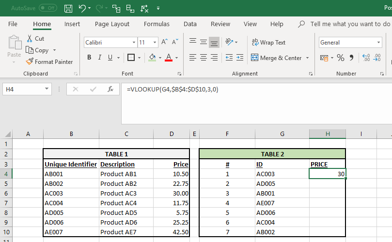
In the example above you can see how the VLOOKUP function is used to return the price of an item from Table 1 to a cell in Table 2 using the Unique Identifier of Table 1 as index.
◉ MAX & MIN
These functions are very simple, just type in the column or row of numbers you want to search following the function and it will output the MAX or MIN value depending on the function you use. For example, =MAX(A1:A10) would output the maximum numerical value in those rows.
◉ AND
This is another logical function in Excel, and it will check if certain things are true or false. In contrast to the IF function above the AND function is used when you want to check more than one condition. For example: =AND(A1=”CORRECT”, B2>10) would output TRUE if A1 is CORRECT and the value of B2 is greater than 10. You can add more conditions with another comma.
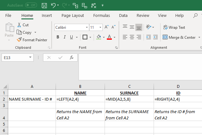
◉ CELL, LEFT, MID and RIGHT
These advanced Excel functions can be combined to create some very advanced and complex formulas to use. The CELL function can return a variety of information about the contents of a cell (such as its name, location, row, column, and more).
The LEFT function can return text from the beginning of a cell (left to right),
MID returns text from any start point of the cell (left to right), and
RIGHT returns text from the end of the cell (right to left).
Below is an illustration of these three formulas in action.
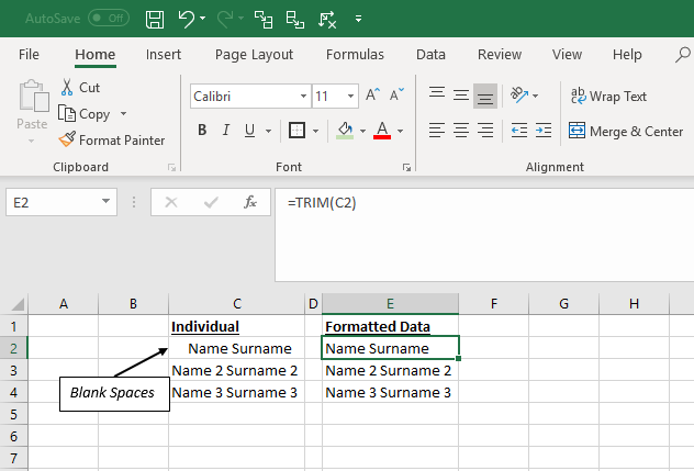
◉ LEN and TRIM
These are a little less common, but certainly very useful formulas in cases you need to organize and manipulate data which are not always perfectly formatted and sometimes there are issues like extra spaces at the beginning or end of cells.
LEN is similar to COUNT but instead of counting the number of values in an array LEN counts the number of characters in a string. i.e. You can use =LEN(A1) to count the number of characters included in A1.
TRIM removes blank spaces from a string to clean up data incorrectly formatted. See below for an example on how this function works.
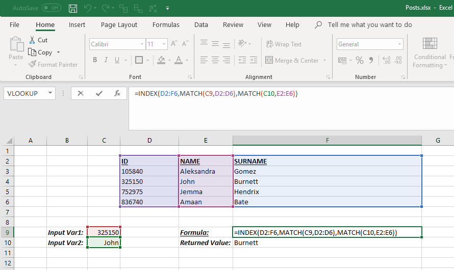
◉ INDEX MATCH
This is an advanced alternative to the VLOOKUP or HLOOKUP formulas (which have several drawbacks and limitations). INDEX MATCH is a powerful combination of Excel formulas that will take your Excel spreadsheets to the next level.
INDEX returns the value of a cell in a table based on the column and row number.
MATCH returns the position of a cell in a row or column.
Here is an example of the INDEX and MATCH formulas combined. In this example, we look up and return a person’s Surname based on their ID and Name. Since Name and ID are both variables in the formula, we can change both.
◉ IF combined with AND / OR
Anyone who’s spent a great deal of time doing various types of financial models knows that nested IF formulas can be a nightmare. Combining IF with the AND or the OR function can be a great way to keep formulas easier to audit and easier for other users to understand.
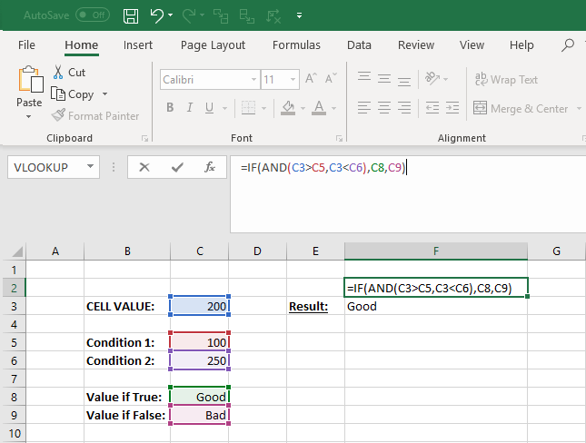
In the example above, you will see how we used the individual functions in combination to create a more advanced formula.